R. Lattuada, and J. Raper
A common method for the reconstruction of a geometric figure given a set of sample points is the use of a triangulation algorithm to connect the points and find the convex hull. In this research, Delaunay triangulation procedures have been used in the reconstruction of 3D geometric figures where the complexity of the problem is much greater than the 2D case. The use of Delaunay triangulations is particularly suited when we do not want to force any constraints on the set of points to be connected. Besides, Delaunay triangulations have some interesting properties as optimal equiangularity and uniqueness ( 2D ).
During the early 1990's one of the most dynamic fields in spatial information science has been the development of three dimensional GIS [RAP89] [RAP 91]. This early work has generated effective techniques for the visualisation and analysis of three dimensional rasters (based on cuboids or voxels) and for the indexing of vector polylines in three dimensional space [TUR91]. However, by contrast, the interpolation of sparse point datasets into coherent and robust models in unseen, structurally complex geoscientific domains remains a central and largely unsolved problem [RAP 95].
This paper reports research into methods of extending triangulation-based interpolation methods from two to three dimensions, suggests hybrid implementation mechanisms to optimise performance and discusses the particular requirements of geoscientific interpolation as they affect the triangulation procedure.
A systematic approach to the problem of connecting a set of points dates back to 1850 and is due to Dirichlet. He proposed a way to subdivide a given domain into a set of convex polygons. Given two points Pi and Pj in the plane T, the perpendicular to the segment PiPj in the middle point divides the plane T into two regions, Vi and Vj. Region Vi contains all and only the points closest to Pi than to Pj ; if we have more points we can easily extend this concept saying that Vi is the region assigned to Pi so that each point belonging to Vi is closest to Pi than to any other point.
The subdivision of the space determined by a set of distinct points so that each point has associated with it the region of the space nearer to that point than to any other is called Dirichlet tessellation.
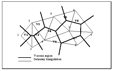
This process applied to a closed domain generates a set of convex distinct polygons called Voronoi regions which cover the entire domain. This definition can be extended to higher dimension where, for example in three dimensions, the Voronoi regions are convex polyhedrons. If we connect all the pairs of points sharing a border of a Voronoi region we obtain a triangulation of the convex space containing those points. This triangulation is known as Delaunay triangulation. An example of the relationship between Voronoi regions and Delaunay triangulation in two dimensions is given in fig. 1. Similarly we can obtain a triangulation for higher dimensions, for example in three dimensions if we connect all pairs of points sharing a common facet in the Voronoi diagram, the result is a set of tetrahedra filling the entire domain.
Fig 1 Voronoi regions and associated Delaunay triangulation
The Delaunay triangulation has some interesting properties [BAK87]:
There are a wide variety of algorithms available to build a Delaunay triangulation for a set of points [KG91]. The one described here and used for this research was first described by Bowyer [BOW81] and Watson [WAT81] and has been proved to be the best of those available in terms of quality of elements generated in three dimensions [KAG91]. This is an incremental algorithm, meaning that points are added one at a time into an existing triangulation and, although described for two dimensions, can be easily extended to three or more. The procedure is totally automated and requires no user intervention.
The algorithm can be described as follows:
Let Tn be the Delaunay triangulation of a set n of points , Vn = {Pi | I = 1,..,n}. By defining a simplex as any n-dimensional polygon and a convex hull as the domain to which these points belong to, is formalised as Rs the radius circumscribed to each simplex S of T and as Qs the centre of the n-dimensional circumscribed sphere. Now we insert a new point Pn+1 in the convex hull of Vn and define B={S | S Tn | d(Pn+1,Qs) < Rs} where d(p,Q) is the Euclidean distance between points P and Q. Now B is not empty as Pn+1 lies in the convex hull of Vn and inside a simplex S1 belonging to Tn, so at least S1 belongs to B. The region C formed when B is removed from T is simply connected, contains Pn+1, and Pn+1 is visible from all the points that form the border of C. It is then possible to generate a triangulation of the set of points Vn+1 = Vn {Pn+1} connecting Pn+1 with all the points that form the border of C : this triangulation is a Delaunay triangulation. For a complete demonstration of the above statements see [BAK87].
It is evident from the definition of a Delaunay triangulation that problems arise in the procedure when certain degeneracies occur in the data.
Common degeneracies in two or more dimensions are :
Common ways to deal with such degeneracy are : reject the point, delay the point insertion, shift its co-ordinates. The choice as to which is the best one often depends on the application; for example rejecting the point may be acceptable if we have a high points density.
For a given set of points in two dimensions, the Delaunay triangulation is univocaly determined and therefore unique, but there are some cases when the triangulation is not unique as there exist different ways of connecting points and all lead to a valid triangulation. This degeneracy is quite common for regular distribution of points, for example in two dimensions when four points lie on a circle and the Voronoi vertexes are coincident.
To efficiently handle geometric objects in triangulations there is the need for data structures supporting efficient operations on the objects and capable of handling queries on attributes or, most important, on the object's position within the domain [BAK89b]. The specific data structure implemented in this work is the N-Tree. This is a generic dynamic n-dimensional tree used to recursively divide the domain and provide efficient operations (mainly search) on geometric objects such as points, edges, triangles and tetrahedra.
This kind of data structure also provides an efficient way of checking object uniqueness; for example when an initial set of points is loaded to be triangulated, the points are all inserted in an N-Tree, duplicate points or points that are equal due to the limited machine precision or rounding error will fall into the same space partition, in this way duplicate points are eliminated and the initial requirement for the Delaunay triangulation satisfied.
The N-Tree data structure is similar to the octree data structure, as they are both recursive space subdivision data structures. However in the N-Tree there is no fixed resolution for the subdivision which means that there is no limit to the number of objects present at any moment in the tree. We can see the octree as a way of representing an object where the model and the data structure are completely synonymous since the data structure is in fact the model. In contrast, the N-Tree is more generic (actually a superset of the octree) as its main use is to store objects rather than represent them. This is true for the basic entities such as points, edges, triangles, and so on. Nevertheless, as the Delaunay triangulation of a domain is stored itself in an N-Tree as a set of geometric entities (tetrahedra or triangles), we can also think of it as a way of representing an object, our domain in this case, with the full advantages of a dynamic data structure. This means that the user can regenerate all or part of the model as desired. The scope to generalise and interpolate features by taking full advantage of the N-Tree data structure is currently being investigated.
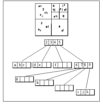
Fig 2 n-tree data structure in two dimensions
Triangulation of a point set is an important method with many applications including finite element simulations. Though a number of algorithms exist for triangulating a point set in two or three dimensions, few of them address the problem of optimising the shape of the triangular elements [BAR91].
To reduce ill-conditioning in simulations as well as discretization errors, finite elements methods require triangular meshes of bounded aspect ratio. The aspect ratio of triangles or tetrahedra is defined as the ratio of the radii of the inscribing circle to that of the circumscribing one (spheres in case of tetrahedra). While in the two dimensional case the Maximum-Minimum angle property (see above) of the Delaunay triangulation guarantees the best possible shape for the elements, this property does not hold in three dimensions [BAR91]. Though several good heuristics have been published [BAR91] [KAG91], to date there is no known algorithm that triangulates the convex hull of a three dimensional point set with tetrahedra of guaranteed qualities e.g. aspect ratio.
The approach taken in this implementation, based on the Bowyer-Watson algorithm which is sound in two dimensions, is to further subdivide the elements (triangles or tetrahedra) adding points so that the shape of the elements obtained after the split is better than that of the original element.
There are several reasons to try to build well shaped elements, triangulations whose elements have very low aspect ratios are undesirable because :
If we think of our model as based on tetrahedral elements with vertices at the given data points, each point has an attribute which can be associated with the tetrahedra using a local piecewise interpolation method (a simple way is to calculate the average of the values of its vertices). Whichever interpolation method we choose to use, it is important that the shape of the tetrahedra reflect the representative location of the attributes if we want good results from the interpolation process.
To define the complexity of the algorithm used we need to highlight which components are dependent on the number of points and therefore play an important part in the definition procedure. When a new point is inserted into an existing triangulation we need to search the list of triangles to find all elements whose circumcircle contains the new point. The time needed to reconnect the points once the elements forming the void are found can be considered constant.
The time needed to triangulate N points can be expressed as : T = (Tk + T1k) where Tk is the time to find the first triangle to be deleted and T1k the time to find all the others.
If we maintain a topological relationship among the elements so that each triangle also stores the reference to all its neighbours we can consider T1k as proportional to the number of elements in the void which is independent from k. With the exception of the first search all other operations are of local nature and may be carried out in a time independent of the number of points currently in the structure. Therefore we can estimate the time complexity of the algorithm as roughly proportional to Tk. The search time Tk will be proportional to k leading to an overall time complexity of O(N2). Using the data structure described in the previous chapter (N-Tree), the cost of the first search can be reduced to O(logN) giving an overall time complexity for the triangulation algorithm of O(NlogN).
The programming language used in this implementation is C++. This is an object oriented programming language well suited to define both geometric objects and data structures. The advantages of using such approach are :
Each separate module is arranged as a library that can be easily linked to any application.
Many forms of geoscientific analysis seek to collect data about spatial objects and domains such as features of the solid earth (aquifers), oceans (currents) or atmosphere (weather fronts), which fill or enclose three dimensional space. A complete geometric representation of these domains requires the definition of each known location in a x, y, z co-ordinate system. If a qualitative representation of the object is required then attributes will have to be linked to the geometric descriptions.
The approaches to three dimensional representation and structuring of geo-objects can be categorised as raster, vector, and function based [JON89]. The raster solutions are mostly based around the voxel, which in not necessarily cubic, as a basic unit. Many authors [POI78] [FLO82] have shown the advantages of terrain modelling based on TINs. Compared to the traditional grid based techniques they allow more adaptive modelling and flexible handling of terrain data. The potential of TIN-based methods has been partly exploited in two dimensions but hardly any work has been done in three dimensions.
There are several reasons to try to describe a geo-model using a three dimensional triangulation :
The major challenge of this research is the representation of relationships and interpolation of sparse geoscientific data. Hence, although all the above triangulation algorithms work well with random data sets, when triangulation points are obtained from solid models or boreholes they are not randomly positioned and will usually form highly degenerate set of points aligned on the z axis which form sub-optimum element shapes. This is why a shape refinement post processing has been applied to the initial set of elements (see figure 3a and 3b).
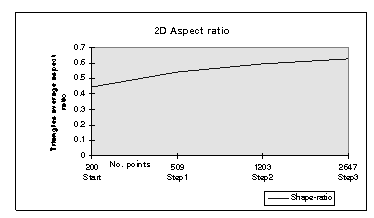
Fig 3a Shape improvement procedure (2D)
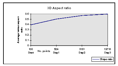
Fig 3b Shape improvement procedure (3D)
To test the approach set out in this paper a typical geoscientific dataset was triangulated using this method. The data was derived from a set of shallow boreholes drilled in a coastal spit feature. The triangulated points were derived by sampling the recovered sediments at 25 cm vertical intervals and making a laboratory determination of the mean particle size. Data points are arranged vertically forming columns of data points; some data points are missing due to non-sample recovery. Note that the vertical sampling interval is approximately 20-30 times the horizontal borehole spacing. Tests using other methods of interpolation in three dimensions often give poor results when there are such constraints.
The following procedures have been applied to the sample dataset ( see figure 4 and figure 5 ) :
The procedures set out in this paper seem to satisfactorily show that triangulation methods can be successfully used to structure and interpolate sparse geoscientific datasets. The future aims of this work are to increase the robustness of the implementation and extend its scope to the following areas:
Further case studies will also be undertaken to optimise these methods for geoscientific research where there is still a relative paucity of procedures for three dimensional interpolation.
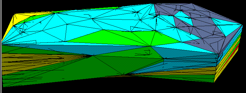
Fig 4 Complete model, attributes are color coded (1).
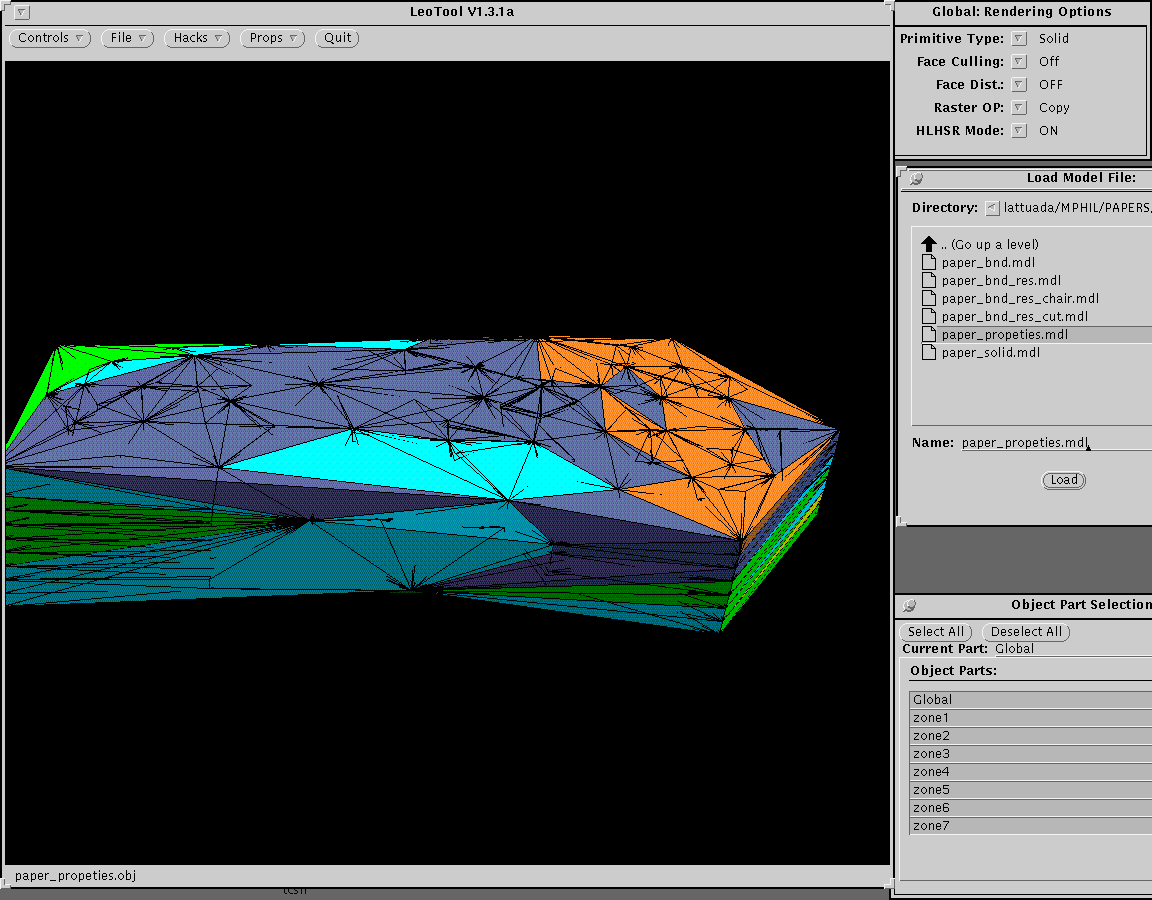
Fig 5 Complete model, attributes are color coded (2).
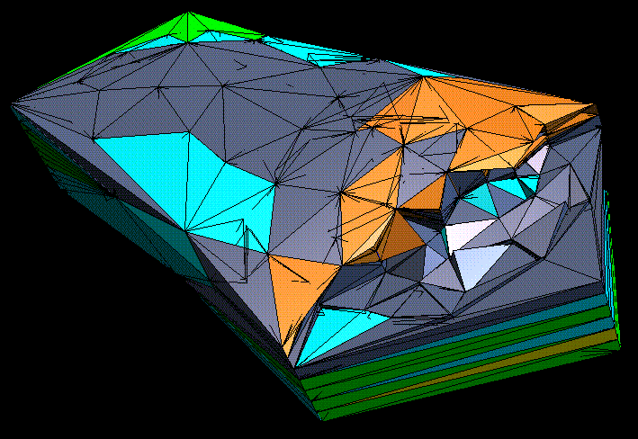
Fig 6 Geometric reselection (chair mode).
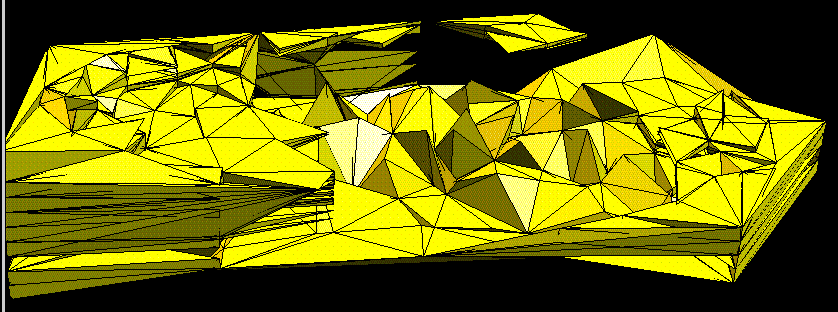
Fig 7 Attribute reselection of 1 layer.
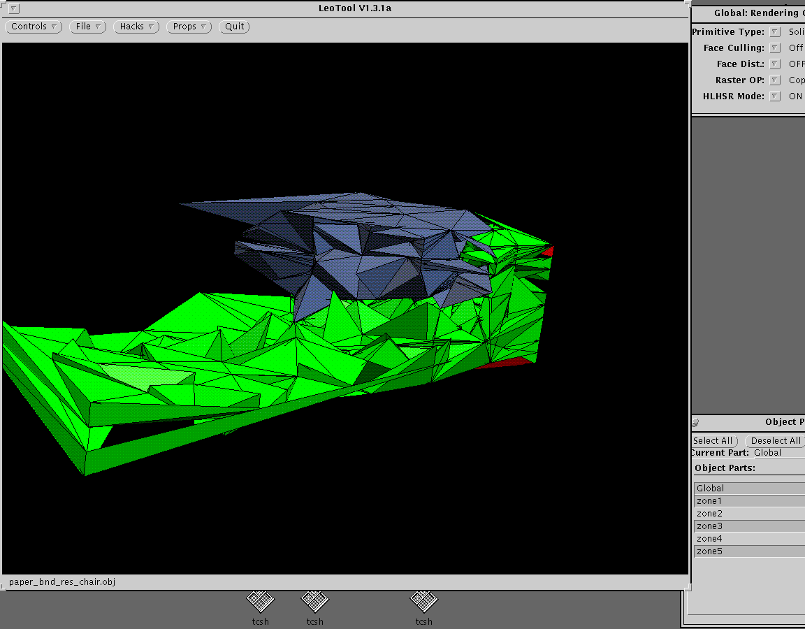
Fig 8 Attribute reselection of 3 layers.
[BAK88] Baker T. J. "Generation of Tetrahedral Meshes Around Complete Aircraft" Second International Conference on Numerical Grid Generation in Computational Fluid Dynamics 1988
[BAK89a] Baker T. J. "Developments and Trends in Three-Dimensional Mesh Generation" Applied Numerical Mathematics (5) 1989
[BAK89b] Baker T. J. "Automatic Mesh Generation for Complex Three-Dimensional Regions Using a Constrained Delaunay Triangulation" Engineering with Computers (5) 1989
[BAK89c] Baker T. J. "Element Quality in Tetrahedral Meshes" 7th International Conference on Finite Element Methods in Flow Problems" 1989
[BAK91] Baker T. J. "Unstructured Mesh Generation and Surface Fidelity for Complex Shapes" AIAA Computational Fluid Dynamics Conference 1991
[BAR91] Barry Joe "Delaunay versus max-min solid angle triangulations for three-dimensional mesh generation" International Journal for Numerical Methods in Engineering, Vol31,987-997, 1991
[BER91] Bern M., Eppstein D., Yao F. "The Expected Extremes in a Delaunay Triangulation" International Journal of Computational Geometry and Applications (1,1) 1991
[BOW81] Bowyer A. "Computing Dirichlet Tessellations" The Computer Journal (24) 1981
[DAV] DavyJ. R., Dew P. M. "A Note on Improving the Performance of Delaunay Triangulation"
[DEY91] Dey T. K., Bajaj C. L., Sugihara K. "On Good Triangulations in Three Dimensions" ACM Communications 1991
[FLO82] De Floriani L., Falcidieno B., Pienovi C. "Triangulated Irregular Networks in Geographical Data Processing", in Rinaldi s. : Enviromental Systems Analysis and Management, pp801,811, 1982
[JAC80] Jackins C. L., Tanimoto S. L. "Oct-Trees and Their Use in Representing Three-Dimensional Objects" Computer Graphics and Image Processing (14) 1980
[JON89] Jones C.B. "Data structures for 3D spatial information systems", International Journal of Geographical Information Systems, 3:15-32
[KAG91] S.Kanaganathan,N.B. Goldstein "Comparison of four point adding algorithms for Delaunay type three dimensional mesh generators", IEEE Transactions on magnetics, Vol 27, No 3, May 1991
[HELLE] Heller Martin "Triangulation algorithms for adaptive terrain modelling"
[LAW86] Lawson L. "Properties of n-dimensional triangulations" Computer Aided Geometric Design (3) 1986
[LEE91] Lee R. C. T., Fu J. J. "Voronoi Diagrams of Moving Points in the Plane" International Journal of Computational Geometry and Applications" 1991
[LOH88] Lohner R. "Some Useful Data Structures for the Generation of Unstructured Grids" Communications in Applied Numerical Methods (4) 1988
[MEA82] Meagher D. "Geometric Modeling Using Octree Encoding" Computer Graphics and Image Processing (19) 1982
[MOO91] Moore D., Warren J. "Bounded Aspect Ratio Triangulation of Smooth Solids"ACM Communications 1991
[PER90] Peraire J., Morgan K., Peiro J. "Unstructured Mesh Methods von Karman Institute for Fluid Dynamics Lecture Series 1990-06
[POI78] Poiker T.K., Fowler J.J., Mark D.M. "The Triangulated Irreguler Network", Proceedings of the Digital Terrain Models Symposium St. Louis, Miss., pp.516-540, 1978
[PRE85] Preparata F. P., Shamos M. I. "Computational Geometry, An Introduction" 1985
[RAP89] Raper,JF (ed.) (1989) Three Dimensional applications in geographical information systems. London: Taylor and Francis.
[RAP91] Raper, JF and Kelk, B (1991) Three dimensional GIS. In Maguire, D Goodchild, M. and Rhind, D. (eds) Geographic Information Systems: Principles and Applications, Harlow: Longman, pp299-317.
[RAP95] Raper, J.F. (1995) Making GIS multidimensional. Proc. 1st Joint European Conf. on Geographic Information, The Hague, Netherlands, 27-31 March 1995, 1, 232-40.
[SAP91] Sapidis N. S., Perucchio R. "Domain Delaunay Tetrahedrization of Arbitrary Shaped Curved Polyhedra Defined in a Solid Modeling System" ACM Communications 1991
[SIB77] Sibson B., Green P. J. "Computing Dirichlet Tessellations in the Plane" The Computer Journal 1977
[SIB78] Sibson B. "Locally equiangular triangulations" The Computer Journal (21) 1978
[TAN83] Tanemura M., Ogawa T., Ogita N. "A New Algorithm for Three-Dimensional Voronoi Tessellation" Journal of Computational Physics (1983)
[TUR] Turner, K. (ed.) Three dimensional modelling with geoscientific information systems , Dordrecht: Kluwer
[VAN91] Vanecek G. Jr. "Brep-Index: a Multidimensional Space Partitioning Tree" International Journal of Computational Geometry and Applications (1,3) 1991
[YER84] Yerry M. A., Shephard M. S. "Automatic Three-Dimensional Mesh Generation by the Modified-Octree Technique" International Journal for Numerical Methods in Engineering (20) 1984
[WAT81] Watson D.F. "Computing the N-Dimensional Delaunay Tessellation with Apllication to Voronoi Polytopes" The Computer Journal (24) 1981
[WEA85] Weatherill P. "The Generation of Unstructured Grids using Dirichlet Tessellations" MAE Rept. No. 1715 Princeton University 1985
[WEA90] Weatherill P. "Numerical Grid Generation" von Karman Institute for Fluid Dynamics Lecture Series 1990-06
Roberto Lattuada is currently a second year part-time research student at the geography department, Birkbeck College, London. He is also working as system developer in an EU GIS project for the management of FMD outbreaks. His interests include: GIS applications, mesh generation, software development. He received a degree in Computer Science from the University of Milan (1991).
Jonathan Raper is a lecturer in GIS in the Department of Geography at Birkbeck College, University of London. His current research interests include spatial languages and user environments for GIS, environmental modelling with GIS, GIS and multimedia (he chairs the ESF GISDATA Task Force on multimedia GIS) and 3D/4D modelling in the geosciences (he was editor of '3D applications in GIS').